Microsoft Excel Project - Vlookup and Hlookup

 

Hey, how are you? Welcome again!!

So now we are moving to some complex functions and formulas, which are Vlookup and Hlookup.

VLOOKUP & HLOOKUP

VLOOKUP is a function to read or find data vertically. The function form is :

    =Vlookup(lookup_value;  table_array; column_index_num; range_lookup)

    "lookup_value": the value as the basic table reading
    "table_array": the range of the reference table
    "column_index_num": the number of the column position on the reference table
    "range_lookup": TRUE for approximate results, or FALSE for accurate results.

HLOOKUP is a function to read or find data horizontally. The function form is :

    =Hlookup(lookup_value;  table_array; row_index_num; range_lookup)

    "lookup_value": the value as the basic table reading
    "table_array": the range of the reference table
    "row_index_num": the number of the row position on the reference table
    "range_lookup": TRUE for approximate results, or FALSE for accurate results.

Electronic Sales Report

Here is my project using the VLOOKUP and HLOOKUP formulas.

Vlookup Hlookup

The first image shows the blank table report.

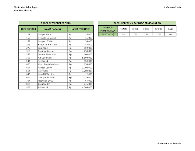
The middle one shows the reference table used in this project.

The last image shows the final report after calculation using the VLOOKUP, HLOOKUP, and other functions and formulas.

FUNCTIONS AND FORMATS

Here are the conditions and functions that I use in this project : 

• Paper size A4
• Landscape orientation
• Margin 2222
• Custom Border and Shading
• Merge and Center for some merge cells
• Cells alignment
• Accounting format number
• Custom Header Footer

CALCULATION

Nama Produk

"Nama Produk" or Product Name was obtained by using the VLOOKUP formula.

Here is the value example of the first row :

    =VLOOKUP(B7;REFERENSI!$A$2:$C$19;2;FALSE)

    "B7": the lookup_value, containing the "Kode Produk" or the Product Code.

    "REFERENSI!$A$2:$C$19": table_array, containing the Reference Table named

                                                       "Tabel Referensi Produk". For easier drag down the formula

                                                       to the below rows, I use absolute reference for this range.

    "2": column_index_num, containing the column number position of the "Nama Barang" or

           Product Name on the "Tabel Referensi Produk" in the Reference Table.

    "FALSE": range_lookup, for accurate results.

Harga

"Harga" or Price was obtained by using the VLOOKUP formula.

Here is the value example of the first row :

    =VLOOKUP(B7;REFERENSI!$A$2:$C$19;3;FALSE)

    "B7": the lookup_value, containing the "Kode Produk" or the Product Code.

    "REFERENSI!$A$2:$C$19": table_array, containing the Reference Table named

                                                       "Tabel Referensi Produk". For easier drag down the formula

                                                       to the below rows, I use absolute reference for this range.

    "3": column_index_num, containing the column number position of the "Harga (Per Unit)" or

           Price each Unit on the "Tabel Referensi Produk" in the Reference Table.

    "FALSE": range_lookup, for accurate results.

Subtotal

Subtotal was obtained by multiplying "Harga" and "Jumlah Unit"

Diskon (%)

"Diskon (%)" or Discount (%) was obtained by using the HLOOKUP formula.

Here is the value example of the first row :

    =HLOOKUP(G7;REFERENSI!$E$2:$J$3;2;FALSE)

    "G7": the lookup_value, containing the "Metode Pembayaran" or the Payment Method.

    "REFERENSI!$E$2:$J$3": table_array, containing the Reference Table named

                                                    "Tabel Referensi Metode Pembayaran". For easier drag down

                                                    the formula to the below rows, I use absolute reference for this range.

    "2": row_index_num, containing the row number position of the "Diskon (%)" or Discount (%)

           on the "Tabel Referensi Metode Pembayaran" in the Reference Table.

    "FALSE": range_lookup, for accurate results.

Diskon (Rp)

"Diskon (Rp)" or the Discount (Rp) was obtained by multiplying (*) Subtotal and "Diskon (%)".

Total Pembayaran

"Total Pembayaran" or the Total Payment was obtained by subtracting (-) the Subtotal with "Diskon (Rp)"

Total Pemasukan

"Total Pemasukan" or the Total Revenue was obtained by summing the "Total Pembayaran" or the Total Payment using SUM.

    =SUM(J7:J16)

    "J7:J16": the range of the "Total Pembayaran" value.

Maksimum

"Maksimum" or the Maximum was obtained by finding the maximum number of "Total Pembayaran using MAX.

    =MAX(J7:J16)

    "J7:J16": the range of the "Total Pembayaran" value.

Minimum

The Minimum was obtained by finding the minimum number of "Total Pembayaran using MIN.

    =MIN(J7:J16)

    "J7:J16": the range of the "Total Pembayaran" value.

Rata-Rata

"Rata-rata" or the Average was obtained by calculating the average value of "Total Pembayaran using AVERAGE.

    =AVERAGE(J7:J16)

    "J7:J16": the range of the "Total Pembayaran" value.